CIT-423 Machine Learing
Professor Md Abdul Masud
References
- Book-1: Ethem Alpaydın - Introduction to Machine Learning (Third Edition)
- Book-2: Tom M. Mitchell - Machine Learning
- Book-3: Ian Goodfellow, Yoshua Bengio, Aaron Courville - Deep Learning - MIT Press (2016)
- Sheet-1: Understanding LSTM Networks - {Web Link} - {PDF}
Introduction
- Concepts on Machine Learning, Deep Learning, and Reinforcement Learning
-
Concepts on Supervised Learning, Unsupervised Learning, and Semi-Supervised Learning
-
Supervised Learning
- Discrete \(\to\) Classification \(\to\) Accuracy
- Continuous \(\to\) Regression \(\to\) Error
-
Prameter Estimation \(\to\) Linear Regression
Chapter 2 : Supervised Learning (Book-1)
Slide: i2ml2e-chap2-v1-0
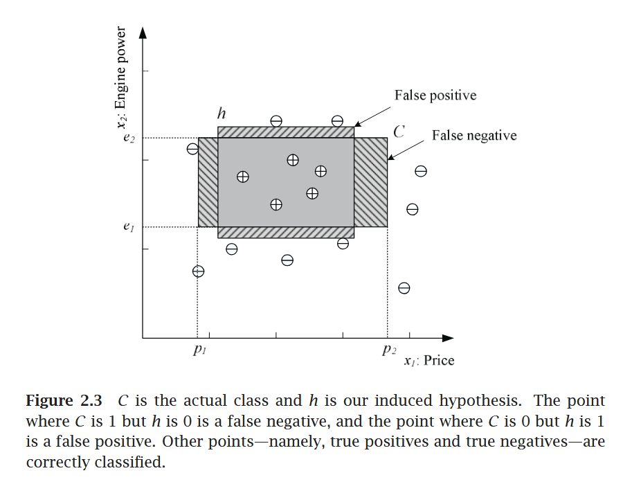
2.1 Learning a Class from Examples (Data)
Classification:
- Hypothesis \(\to\) Equation/Mathematical Model
- Most specific hypothesis \(\to\) tightest hypothesis + all positive
- Most general hypothesis \(\to\) largest hypothesis
Assignment
Multi-Class Classification
- Confusion Matrix
- Accuracy
- Precision
- Recall
- F1-Score
- ROC Curve
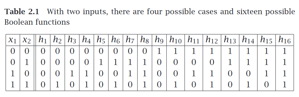
2.2 Vapnik-Chervonenkis (VC) Dimention
- largest point
- n points \(\to\) \(2^n\) possible points
- \(\tau = {f(x)}\)
2.3 Probably Approximately Correct (PAC) Learning
Given a class, \(C\), and examples drawn from some unknown but fixed probability distribution, \(p(x)\), we want to find the number of examples, \(N\), such that with probability at least \(1 − δ\), the hypothesis \(h\) has error at most \(\epsilon\), for arbitrary \(δ ≤ 1/2\) and \(\epsilon > 0\)
where \(CΔh\) is the region of difference between \(C\) and \(h\)
2.4 Noise
2.5 Learning Multiple Classes
In the general case, we have \(K\) classes denoted as \(C_i, i = 1, . . . , K\), and an input instance belongs to one and exactly one of them. The training set is now of the form \(X = \{x^t , r^t \}N t =1\) where \(r\) has \(K\) dimensions and
We have \(K\) hypotheses to learn such that,
The total empirical error takes a sum over the predictions for all classes over all instances:
2.6 Regression
- The function is not known but we have a training set of examples drawn from it, where \(r^t ∈ \mathbb{R}\). If there is no noise, the task is interpolation.
-
We would like to find the function \(f(x)\) that passes through these points such that we have \(r^t = f(x^t)\)
-
In polynomial interpolation, given \(N\) points, we find the \((N−1)\)st degree polynomial that we can use to predict the output for any \(x\). This is called extrapolation extrapolation if \(x\) is outside of the range of \(x^t\) in the training set.
-
In regression, there is noise added to the output of the unknown function where \(f(x) ∈ \mathbb{R}\) is the unknown function and is random noise.
- The explanation for noise is that there are extra hidden variables that we cannot observe where \(z^t\) denote those hidden variables.
- The empirical error on the training set \(X\) is
- Our aim is to find \(g(·)\) that minimizes the empirical error.
- There we used a single input linear model where \(w_1\) and \(w_0\) are the parameters to learn from data.
- The \(w_1\) and \(w_0\) values should minimize where \(\bar{x} = \sum_{t} x^t /N\) and \(\bar{r} = \sum_{t} r^t/N\)
Assignment
Errors and Evaluation Metrics for Regression
2.7 Model Selection and Generalization
2.8 Dimensions of a Supervised Machine Learning Algorithm
- Loss function, \(L(·)\), to compute the difference between the desired output, \(r^t\), and our approximation to it, \(g(x^t |θ)\), given the current value of the parameters, \(θ\). The approximation error, or loss, is the sum of losses over the individual instances
- Optimization procedure to find θ∗ that minimizes the total error
Chapter 3 : Baysian Decision Theory (Book-1)
unobservable variable
3.2 Classification
Eq. 3.5
3.3 Losses and Risks
--
Chapter 4 : Parametric Methods (Book-1)
Slide: i2ml2e-chap4-v1-0 Parametric Methods
-
How to estimate probabilities from a given training set?
-
Probability density function
- probability mass function
- likelihood vs posterior
4.2
4.2.2 Multinomial Density
(self study)
4.3 Evaluatind an Estimator : Bias and Variance
4.5 Parameter Classification
Fig 4.2, 4.3
4.6 Regression
4.7 Tuning Model Complexity: Bias/Variance Dilemma
Fig 4.5, 4.6
4.8 Model Selection Procedure
fig 4.7
Assignment on Model Selection Criterion
- AIC & BIC information critarion
- Minimum description length
- Baysian model selection process
- Baysian Estimator \(\to\) from Bayes Rules
- Maximum Posterior Estimator
Chapter 5 : Multivariate Methods (Book-1)
5.1 Multivariate Data
5.2 Parameter Estimation
5.3 Estimation of Missing Values
5.4 Multivariate Normal Distribution
fig 5.1
All Equations \(\star \star \star\)
5.11
fig 5.2
Chapter 4 : Artificial Neural Networks (Book-2)
Introduction
Biological Motivation
4.4 Perceptron
4.4.1 Representational Power of Perceptron
4.4.2 The Perceptron Training Rule
4.4.3 Gradiant Descent and The Delta Rule
4.4.3.1 Visualization of Hypothesis Space
4.4.3.2 Derivation of the Gradiant Descent Rule
Table 4.1
- Stochastic Approach to Gradiant Descent
- Limitation of Gradiant Descent Algorithm
- Solution of Gradiant Descent Algorithm
T 4.1
T 4.2
4.5 Multilayer Network and The Back Propagation Algorithm
fig 4.5
4.5.1 Differentiable Threshold Unit
Why perceptron rule is unsuitable for g. D algorithm?
Solution: Sigmoid Unit/ Logistic Function
4.5.2 Back Propagation Algorithm
Table 4.2
4.5.3 Derivation of Back Propagation Rule
figures from 4.6.4 and 4.6.5
Chapter 9 : Convolutional Networks (Book-3)
Neural Network \(\to\) DL
- Forward Propagation
- Backwork Propagation
9.1 The Convolution Operation
fig 9.2
fig 9.11
- Input image \(\to\) Kernel \(\to\) Convolution \(\to\) ReLU
- Feature Mapping
- Deature Extension
- Classification
- Probabilistic Distribution \(\to\) Class/Output (Softmax)
Definitions:
- Stride
- Pooling
- Padding \(\to\) Border problem solve
Example:
o = (i-k)+1
Assignment
Different CNN Variants Different Activation Methods
Deep Learning for Sequence Data
Recurrent Neural Network (RNN)
Problem:
- long term dependency problem
- An unrolled Recurrent Neural Network \(\to\) fig
- small gap: The cloud are in the _
- More Content: _, _, _
Understanding LSTM Networks (Sheet-1)
Figures
LSTM Networks (Book + Website)
The repeating module in a standard RNN contains a single layer.
Core idea behind LSTM
Gate \(\to\) Information \(\to\) Through/Remove
Step by step LSTM work though
Varient of LSTM \(\to\) Assignment
Muhtasim
References
- Model Selection: Overfitting vs. Underfitting: A Complete Example
- L-01.pdf: Overfitting and Underfitting
- Lecture 12: Bias-Variance Tradeoff
- Lecture8.pdf: Nonparametric Methods Recap..
- Clustering.pdf: Unsupervised learning Clustering
- Cluster Analysis
Topics of Lecture - 01
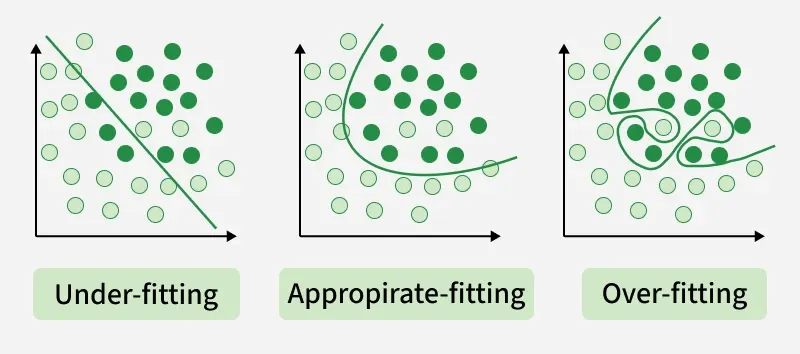
- Overfitting-Underfitting
- Training and Testing Data
- Model Building
- Graphs of polynomial function
- Example: Linear Regression
- Overfit-Underfit
- Example: Logistic Regression
- Training vs Testing Performance
- Bias-Variance Tradeoff
- Error derivation won't be in exam.
- Figure-1
- Figure-2
Topics of Lecture - 02
Model Selection
- Validation
Lecture8.pdf
- Estimating generalization error
- till: Page-31 (Practical Issues in Cross-validation)
Cluster Analysis (Slide)
- till: Slide-66 (Hierarchical Clustering: Problems and Limitations)
Clustering.pdf
- till: Hierarchical Clustering (relevant page)